Statistical Mechanics

Biological Macromolecule Simulation lysozyme in water

Objective

The objective of this project was to demonstrate the process, results and analysis of a Classical Molecular Dynamics (MD) simulation and analysis of a biological macromolecule, in this case a protein, in an aqueous environment. We refer to these simulations as Classical Molecular Dynamics since only Classical Newtonian Dynamics (Equations of Motion) are used. No Quantum or Reactive processes are utilized.

Background

Proteins are nature’s universal machines. For example, they are used as building blocks (e.g. collagen in skin, bones and teeth), transporters (e.g. hemoglobin as oxygen transporter in the blood), as reaction catalysts (enzymes like lysozyme that catalyze the breakdown of sugars), and as nano-machines (like myosin that is at the basis of muscle contraction). The protein’s function is intimately linked to internal dynamics. Therefore, if we want to understand protein function, we often first need to understand its dynamics. Unfortunately, there are no experimental techniques available to study protein dynamics at the atomic resolution at the physiologically relevant time resolution (that can range from seconds or milliseconds down to nanoseconds or even picoseconds). Therefore, computer simulations are employed to numerically simulate protein dynamics.

Therefore, we use the GROMACS MD simulation package for this particular example. This will be a simulation system containing Lysozyme in a box of water, with ions.

The Process

Acquire Protein Structure

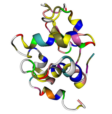
First we must obtain the protein structure. This is normally acquired through the use of database repositories of existing structure files. In this case we will download the protein structure file we will be working with from the RCSB (Research Collaboratory for Structural Bioinformatics) Protein Data Bank. For this tutorial, we will utilize hen egg white Lysozyme (1960 atoms) as seen here (click on the image for a 3D PDF model – you must have Adobe Reader or its equivalent installed). Go to the RCSB website and download the PDB text for the crystal structure using the PDB code 1AKI.

We download the PDB file and then use the GROMACS utility pdb2gmx is to generate three files: the topology for the molecule, a position restraint file and a post-processed structure file. Virtually all MD simulations require the specification of how the atoms interact with each other. In this case we choose to use OPLS-AA/L all-atom force field (2001 amino acid dihedrals). The files produced by pdb2gmx contain the information which includes the force field information, including non bonded parameters (atom types and charges) as well as bonded parameters (bonds, angles, and dihedrals).

The topology contains all the information necessary to define the molecule within a simulation. The post-processed structure file is a GROMACS-formatted structure file that contains all the atoms defined within the force field (i.e., H atoms have been added to the amino acids in the protein). The position restraint file is used during initial system equilibration processing to ensure superfluous molecular distortions or collisions do not occur and cause the computational equilibration of the system to fail.

Build the System to be Simulated

MD simulations utilize periodic boundary conditions in order to replicate the behavior of Macroscopic Systems from the simulation of an (in theory, infinitely replicating) unit cell consisting of Atomistic/ Molecular systems. In this case, we will use as our unit cell a cubic box. We will define the box using the GROMACS utility editconf where we will define the protein to be centered in the box with a minimum distance of any part of the protein defined to be at least 1 nm. This is critical since we will be using periodic boundary conditions which require we must satisfy the minimum image convention. I.e., a protein should never see its periodic image, otherwise the forces calculated will be spurious. Specifying a solute-box distance of 1.0 nm will mean that there are at least 2.0 nm between any two periodic images of a protein. This distance is normally judged to be sufficient for just about any cutoff scheme commonly used in simulations.

While protein simulations in vacuo may be of interest to some, in our case we are interested in biologically relevant simulations. Thus, we must solvate the protein in its unit cell. For this case we use (of the myriad water models available) the SPCE model, for convenience. It is a relatively simple model that, in the main, does a reasonable job of representing water and its interactions with other chemical/ physical species. We perform the solvation using the GROMACS utility genbox. We must also realize that the Lysozyme molecule has a charge of +8. So, to get a physically realistic system, we must add counter ions to arrive at a neutral charge system. That is done using the GROMACS utility genion which will replace water molecules with, in this case, Cl- ions.

The resulting system contains 1 protein, 8 Cl- ions, and 10,824 water molecules for a total of 34,440 atoms. The unit cell looks like this (click on the image for a 3D PDF representation):

Prepare the System for Simulation

We now have a solvated, electrically neutral unit cell prepared. The next step is to perform an energy minimization. We must do this to ensure that the system has no steric clashes or inappropriate geometry. If we expect to get physically reasonable results, dynamics cannot be performed prior to this.

We use the GROMACS utility grompp to assemble all the relevant information into a binary input file for use by the GROMACS MD engine, mdrun. We then run a maximum 50000 step simulation, with a step size of 1 femtosecond (fs) The intent is to allow the system to evolve into an equilibrium state at T = 0o K where the potential energy (Epot) should be negative, and (for a simple protein in water) on the order of 105-106, depending on the system size and number of water molecules. The maximum force, Fmax, should be no greater than 1000 kJ mol-1 nm-1.

In our case we obtained the following results:

Steepest Descents converged to Fmax < 1000 in 979 steps
Potential Energy = -6.0590738e+05
Maximum force = 9.4059546e+02 on atom 736
Norm of force = 1.9577955e+01

which is just fine. The energy minimization trend looked like this:

Equilibration

Now that we have assembled the unit cell of the system of interest, we must bring the solute(s) and solvent into a equilibrium state at the desired temperature. The solute and solvent must also be allowed to assume their preferred orientation about each other to ensure the system is physically rational for production MD simulation and analysis.

To assure the probability of success, there are usually two stages of equilibration. The first is a 100 picosecond MD run with an NVT ensemble (constant Number of particles, Volume, and Temperature). This ensemble is also referred to as “isothermal-isochoric” or “canonical.” We use this ensemble as it is the most efficacious way to take the system from it’s minimized energy (low temperature) state to our desired state of T = 300° K. The essential result to be examined, to ensure equilibration is complete, is the Temperature and it’s stability around the desired set point. We use the velocity rescaling thermostat improvement upon the Berendsen weak coupling method, which did not reproduce a correct kinetic ensemble.

Here are the results of that NVT Equilibration:

As we can see, the Temperature has equilibrated quite well to its desired set point of 300o K. Now we can continue with the second phase of Equilibration, i.e. the NPT equilibration.

In the laboratory, experimental conditions usually include a fixed pressure P, temperature T, and number of atoms N. In the NPT ensemble, Number of particles, Pressure and Temperature are kept constant. The NPT ensemble is used for comparison of MD simulations with experiments and thus represents a preferred ensemble for final equilibration. We use it to ensure the unit cell is properly sized per the desired pressure, i.e. 1 bar, the pressure is stabilized at that value and that the density is stabilized at the proper value, i.e. 1000 kg m-3. Only after that is accomplished can we proceed to final, production MD. Pressure coupling is achieved using the Parrinello-Rahman barostat. We will run a 300 ps MD NPT equilibration using the NVT equilibration results as the starting point. 300 ps was chosen due to ensure good system equilibration.

Here are the Cell, Pressure and Density results of that NPT Equilibration:

Production MD

With the Equilibrations concluded, we now can run our production MD. We will run for 2 nanoseconds (2000 ps) using the results of the NPT Equilibration as our starting point.

Following is a summary of the pertinent results.

First, let’s be sure the Temperature is stable:

Temperature is still stable at 300o K with normal variability (0.5% RMSD) and essentially no drift (0.007% from GROMACS averaging and 0% .from the Trend Line through the data).

What about Energy?

Energy is stable with normal variability (0.2% RMSD) and essentially no drift (0.03% from GROMACS averaging and 0% .from the Trend Line through the data).

Cell size is fine.

Pressure:

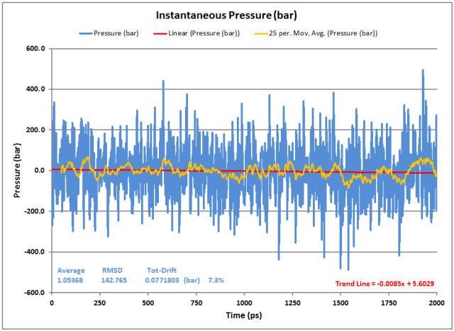
As usual, the instantaneous pressure fluctuates, but this is normal. The moving average helps show the stability of the overall result. The Average pressure is fine at close to 1 bar with very little drift (both from the GROMACS averaging as well as the data Trend Line).

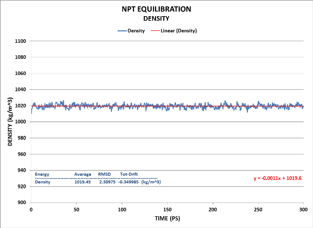
Finally, the Density:

Density fluctuation is minimal as is its drift. Its value is quite close to the target of 1000 kg/m^3.

An important point to make here, is that the MD Production Simulation is interesting but is only a means to an end. It is, in essence, an experiment carried out under very tightly controlled conditions. But, like any other experiment, the results must be analyzed and interpreted to have any meaning. Otherwise, it is just a collection of interesting pictures.

Analysis

Our objective in this study was to show how we do a MD simulation and also to analyze what happens to the object of that simulation (Lysozyme) when it is subjected to the conditions imposed by the simulation experiment.

Here is a view of the actual dynamics during the Production Run. We’re using YouTube as the video server, so set the resolution on the progress bar to HD to get the best viewing results.

Here we can see that the we can see the protein and its surroundings undergo thermal fluctuations. However, the protein structure is stable, which we would expect in the benign environment and at this temperature.

Another measure of protein structural stability can be computed by looking at how far and how fast the Root Mean Square Deviation (RMSD) of the protein occurs during the process of the simulation. One case is the RMSD of the complete protein during the simulation from its initial equilibrated structure. Another is the RMSD of the complete protein from its original experimental (or crystal) value. We can also use the backbone of the protein as a similar comparator in a similar fashion. Those results are seen here:

Both plots show the RMSD is small, (within the levels expected of a protein like Lysozyme at this temperature) levels off and stabilizes quickly thus indicating the structure is stable.

The Radius of Gyration (Rg) of a protein is a measure of the compactness of its organization or folding. If a protein is well organized and folded stably, it will maintain a relatively steady value of Rg. If a protein tends toward disorganization or it unfolds, its Rg will change significantly over time. Here is the Radius of Gyration result for our simulation:

We find the Rg small and stable in value, thus indicating the stable nature of the compactness of the protein over time in our simulation.

Although the Rg is small and stable, it is also advisable to look at the fluctuation in RMS values at the various residues in the protein to see how the internal flexibility varies. If we do that, we find:

where the residues in red are of particular interest. We can view a “flexibility heat map” of the protein:

where the red, orange, and green areas are relatively flexible while the blue regions are relatively rigid (click on the image for a 3D PDF representation).